Accurate magnitude estimates in SeisComP

Precise measurement of amplitudes and calculation of magnitudes for small seismic events observed at local distances have long posed challenges, yet remain crucial for both real-time and non-real-time earthquake monitoring. Recent advancements in SeisComP, particularly in versions 5 and 6, provide new means which may significantly enhance the accuracy of such measurements, thereby elevating the quality of earthquake catalogues.

When dealing with earthquakes or other seismic sources observed at local distances, magnitude types such as ML, MLv, MLc, or MN are of paramount importance. To facilitate more precise calculations of these magnitudes, a tool box of processing and configuration options is now available:

• Amplitude filtering: Amplitudes can now be measured on pre-filtered seismograms, effectively reducing the impact of noise, such as that from microseisms.
• Time windows: Distinct distance-dependent time windows, based on tailored travel-times, enable the exclusion of signals arising from unwanted phases like Rg.
• Quality checks: Automatic assessment of the signal-to-noise ratio helps filtering out amplitude measurements of low quality.
• Regionalization: Regionalization of magnitudes allows for the application of constraints and magnitude calibration functions tailored to specific geographic regions.
• Magnitude aliases: Magnitudes can be derived from others and configured according to specific requirements.

For a comprehensive understanding of amplitude measurements and magnitude calculations within SeisComP, detailed documentation is available online at online documentation of SeisComP .

In the following we demonstrate the potential of tailored amplitudes measurements for ML magnitude. The processing can be similarly applied to other magnitudes such as MLv, MLc or MN.

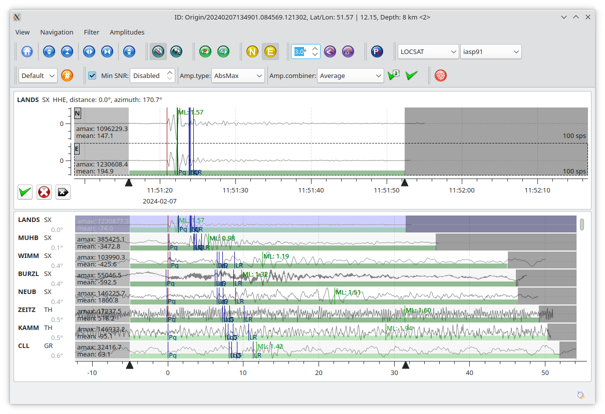
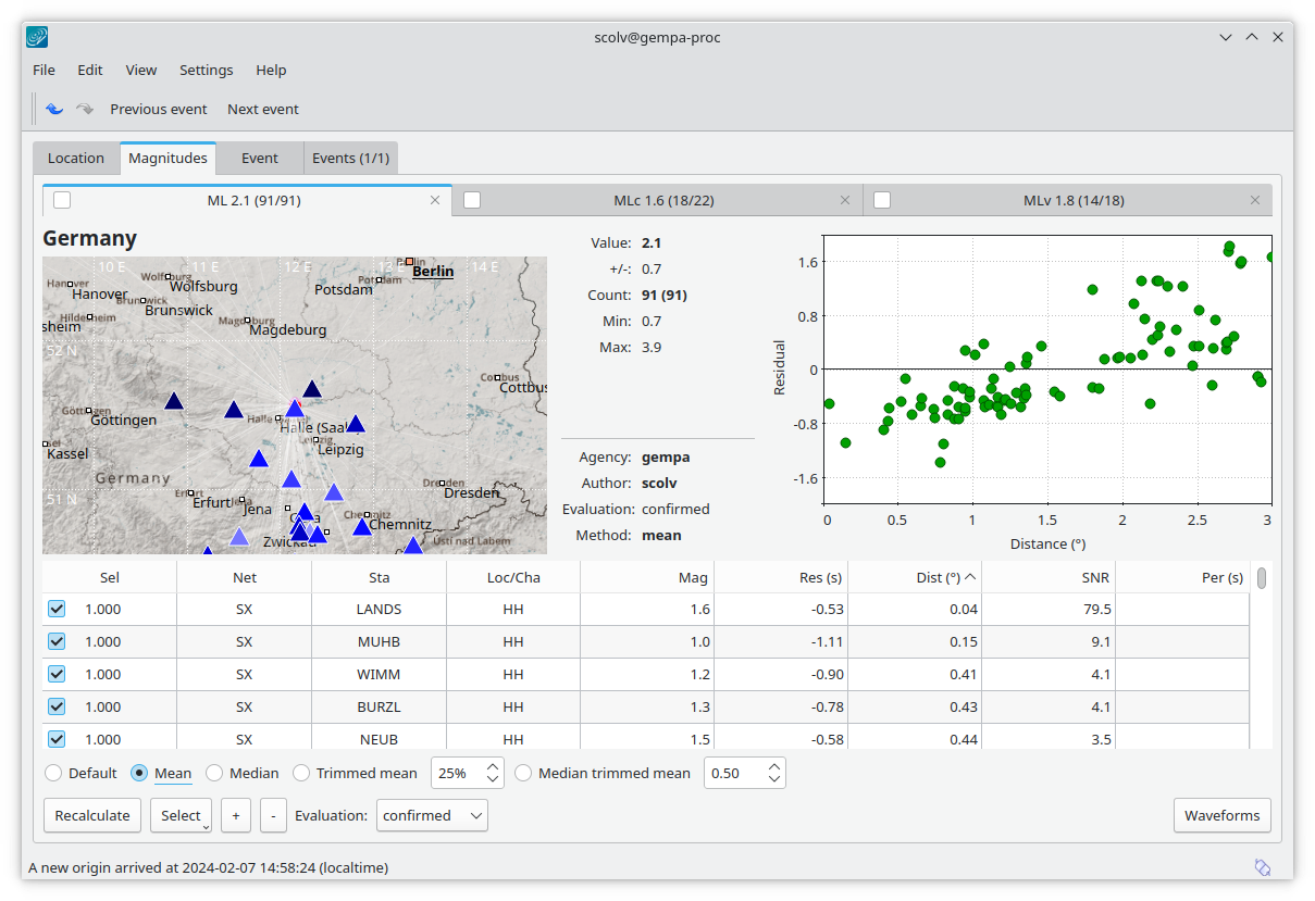
ML Magnitudes from default processing

By default, time windows for measuring ML amplitudes are set to be relatively large to accommodate sizable events with extended source-time functions. However, in this default setting, signal-to-noise ratios are not evaluated, and noise from sources such as microseisms remains unfiltered. Consequently, amplitudes may be measured on phases that are not suited for calibration curves, potentially leading to inaccuracies. Moreover, station magnitudes of small events might exhibit bias at greater distances, consequently inflating network magnitudes beyond their actual values.

scolv amplitude picker. Measurements are made with default parameters.

scolv magnitude tab with station and network magnitudes from amplitudes measurements with default parameters.

ML Magnitudes from tuned processing

Where magnitudes of small events shall be correctly estimated, correctly configured amplitude measurements and magnitude computations are inevitable. Well-tuned amplitudes measurements for correct magnitudes will make a significant difference to the reliability and quality of your event catalogs!

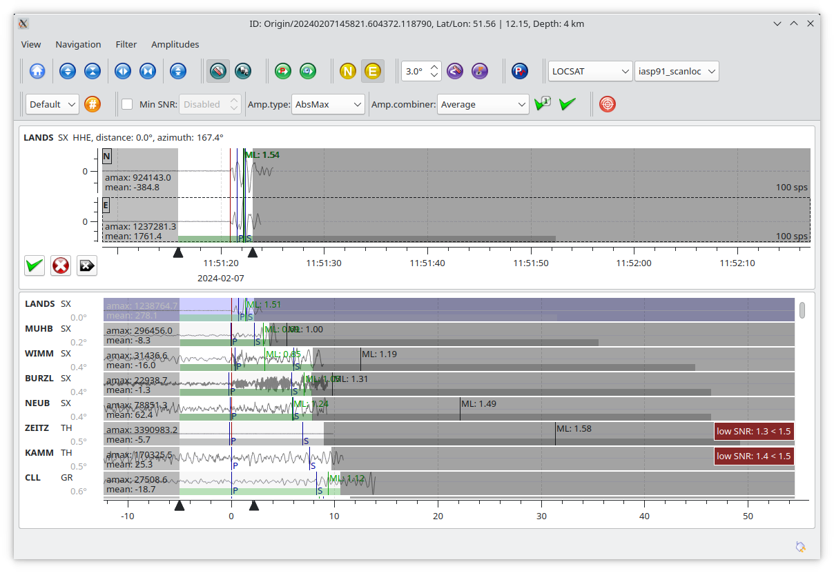
Amplitudes: Precise time windows and quality check

Let’s start with precise time windows for measuring amplitudes and a simple check of the signal-to-noise ratio. In the example below, the default iasp91 profile of LOCSAT is considered for estimating the arrival time of phases. By applying the newly-developed time grammar of amplitude-time windows in global bindings the end time of the signal window is set to either the expected arrival time of the Rg or the epicentral distance measured in degree times 30 s/deg effectively added to origin time, whatever is earliest as given by the function min(). Here, min() is needed since arrival estimates of Rg are only available for shallow events as you can learn from the corresponding travel-time table that must be available. The tables for LOCSAT are stored in @DATADIR@/locsat/tables/. 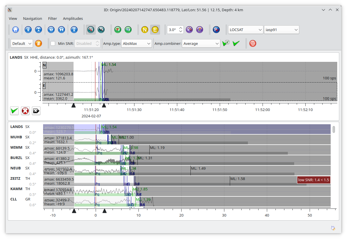Incorporating an additional moderate check of the signal-to-noise ratio (SNR) effectively filters out a substantial portion of amplitudes primarily derived from noise.

Global module configuration:

amplitudes.ttt.interface = LOCSAT
amplitudes.ttt.model = iasp91

Global binding configuration:

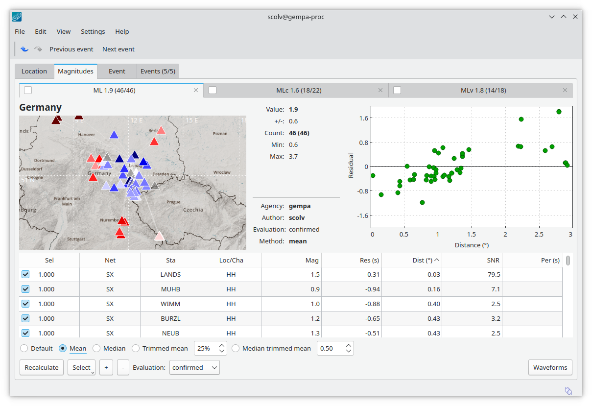
amplitudes.ML.signalEnd = min(OT+D*30,tt(Rg))
amplitudes.ML.minSNR = 1.5

As a result of this configuration, the ML magnitude estimate drops from 2.1 (previously) to only 1.9. Yet, a few outliers persist visibly resulting in a trend towards larger station magnitudes at greater distances.

scolv amplitude picker. Measurements are made with tuned time window and SNR check.

scolv magnitude tab with station and network magnitudes from amplitudes measurements with tuned time window and SNR check.

Amplitudes: Additional pre-filtering

In the provided example, the SNR check is deliberately kept moderate to prevent the loss of small-amplitude measurements. However, the high-frequency amplitudes due to small events may still be hidden in low-frequency noise. We therefore apply an additional high-pass filter before the simulation of Wood-Anderson torsion seismographs, a step essential for standard ML computations.

Global module configuration:

amplitudes.ttt.interface = LOCSAT
amplitudes.ttt.model = iasp91

Global binding configuration:

amplitudes.ML.signalEnd = min(OT+D*30,tt(Rg))
amplitudes.ML.preFilter = BW_HP(3,0.8)
amplitudes.ML.minSNR = 1.5

The high pass filter effectively removes noise due to microseisms. The resulting network ML reduces further to 1.6. Of course such filtering must be applied with care and consistency to avoid underestimation of the magnitudes of larger events.

scolv amplitude picker. Measurements are made with filtered waveforms, tuned time window and SNR check.

scolv magnitude tab with station and network magnitudes from amplitudes measurements with filtered waveforms, tuned time window and SNR check.

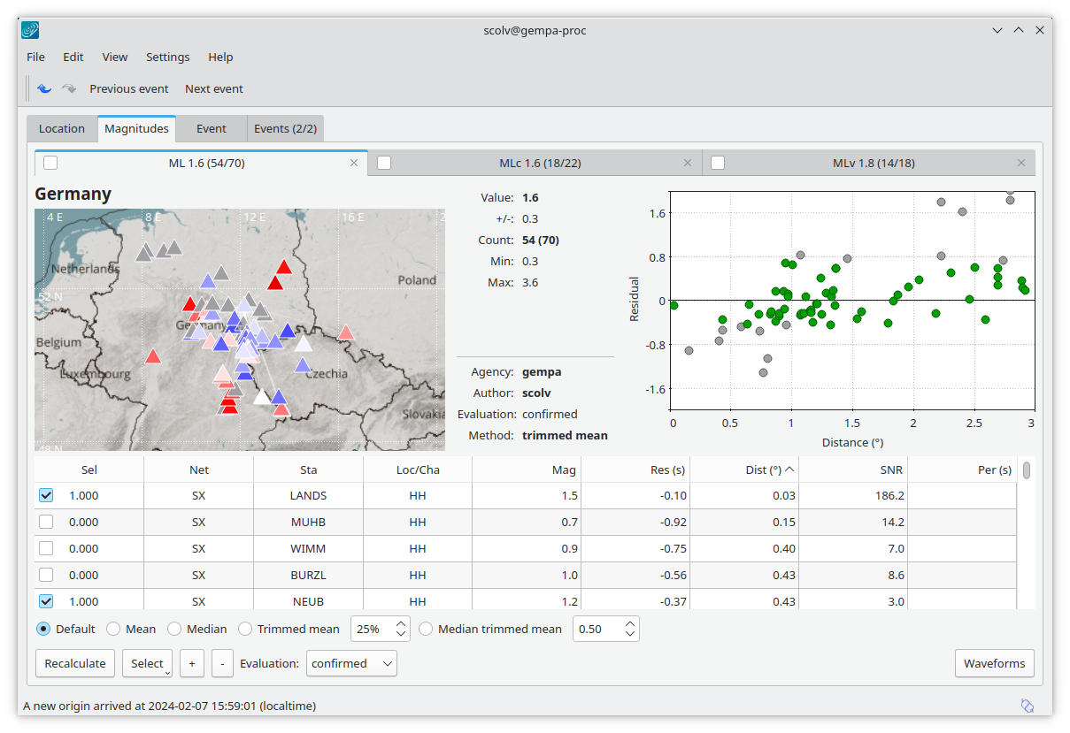
Magnitudes: Calibration functions, regionalization, aliases

While the aforementioned processing focuses on the measurement of amplitudes, a careful selection of the magnitude type itself is definitely worth more considerations. Standard ML and MLv consider epicentral distance between event and observing stations for applying non-parametric calibration formulas. The more recently developed MLc magnitude type , derived from ML, offers great flexibility by allowing to choose between epicentral or hypocentral distances and the option to choose between non-parametric or parametric calibration functions depending on how you have made your calibration.

Furthermore you may choose regionalization , a region-dependent configuration of your magnitude calibration. And if this isn’t enough yet, you can, as of SeisComP in version 6, create magnitude aliases where you may apply different configurations for the same amplitude and magnitude type or even combine and configure a magnitude of one type with an amplitude of another type.

Regionalization and magnitude aliases are now easily configurable through global module parameters. It’s important to note that these configurations need to be set on all machines, including both your server and clients, as they are not automatically communicated from the server to the clients through bindings.